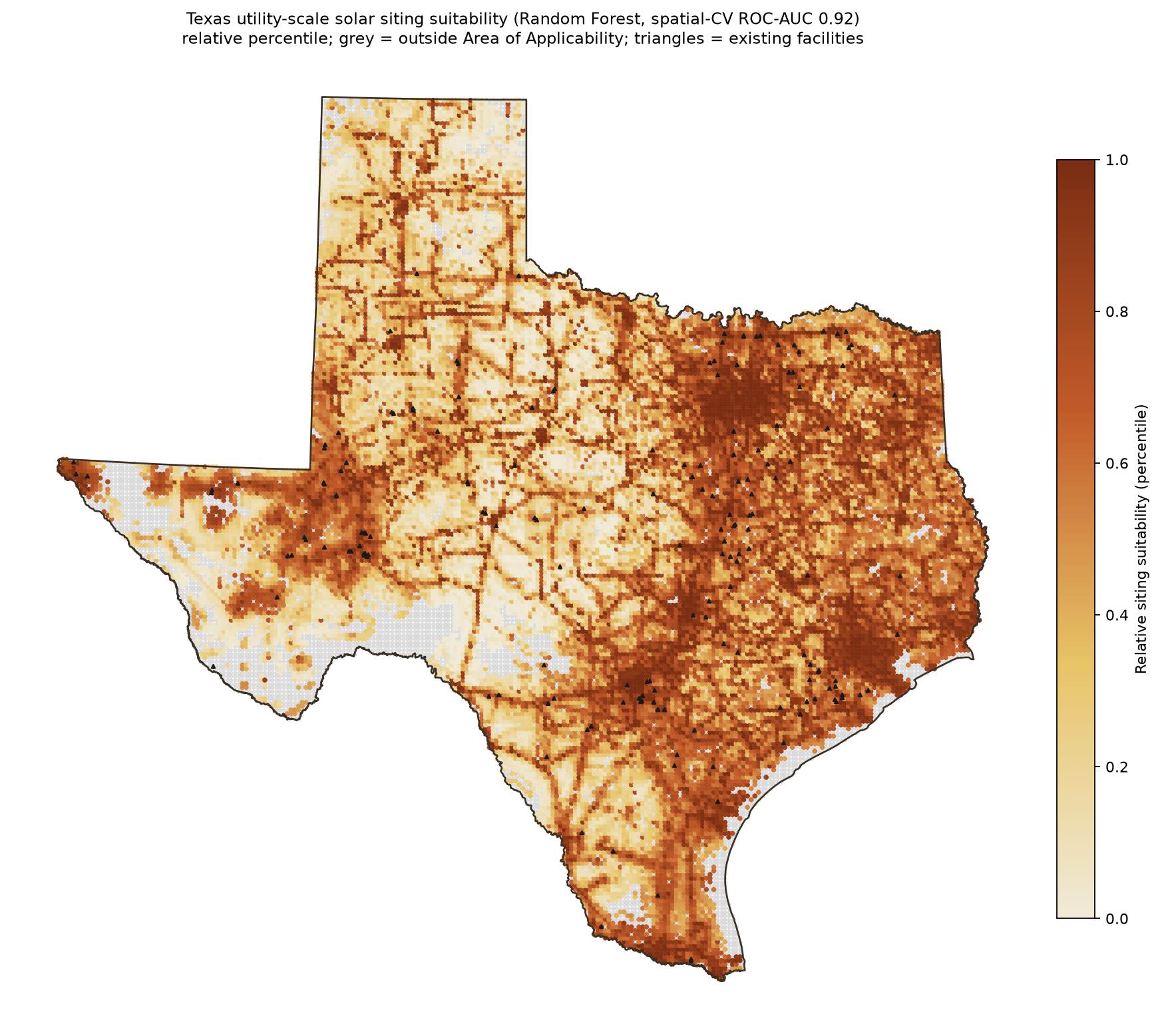
Most solar suitability maps rank land by sunshine and slope. That describes physical potential. Operating facilities follow a different logic.
I modeled realized siting instead: 176 ground-mounted Texas facilities of 1 MW or more (1–500 MW AC, installed 2010–2025), compared against land developers passed over, to see which factors separate the two.
The question is what drives siting decisions in practice, and whether the same rule holds in a state with a completely different energy policy.
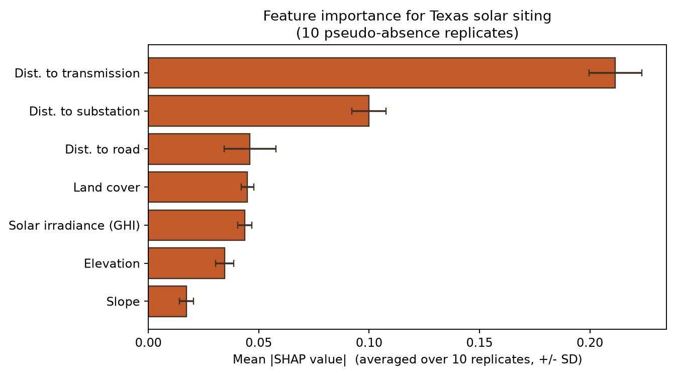
Texas irradiance sits in a narrow, uniformly high range (4.5 to 5.87 kWh/m²/day), so the sunshine difference between one parcel and the next barely moves siting. Distance to transmission infrastructure dominates: about 9× more important than irradiance by permutation importance, 5× by SHAP.
Irradiance still carries real signal; a Boruta shadow-feature test confirms it beats randomized shadow features. It is simply a minor predictor next to grid access.
| Feature | SHAP importance |
|---|---|
| Distance to transmission | 0.212 |
| Distance to substation | 0.100 |
| Distance to road | 0.046 |
| Land cover | 0.045 |
| Solar irradiance (GHI) | 0.044 |
| Elevation | 0.035 |
| Slope | 0.017 |
Transmission ranks first in all 10 replicate draws; irradiance sits in a tangled middle cluster with land cover and roads.
A single-state finding is just a single state. So I applied the Texas-trained model, unchanged, to North Carolina, where the solar economy is the reverse of Texas's: many small plants driven by federal PURPA and state renewable-portfolio policy, on lower irradiance, versus Texas's few large merchant-scale plants.
North Carolina has built roughly four times as many utility-scale solar facilities as Texas despite worse sun (753 vs 176 in USPVDB). Texas dominates on installed megawatts; North Carolina dominates on the number of individual siting decisions, which is the unit this model predicts. The model transfers partially (ROC-AUC 0.76 ± 0.01). Grid access matters in both states, but the operative distance shifts: Texas plants hug transmission at a median of 55 m, while North Carolina's sit near 850 m because they connect to distribution rather than high-voltage transmission.
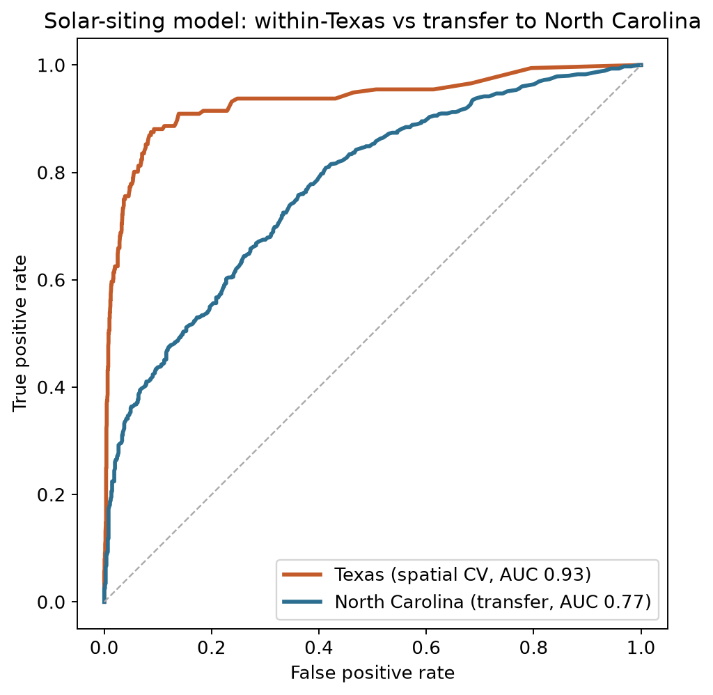
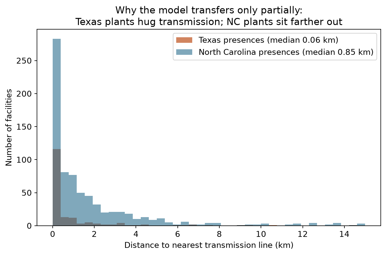
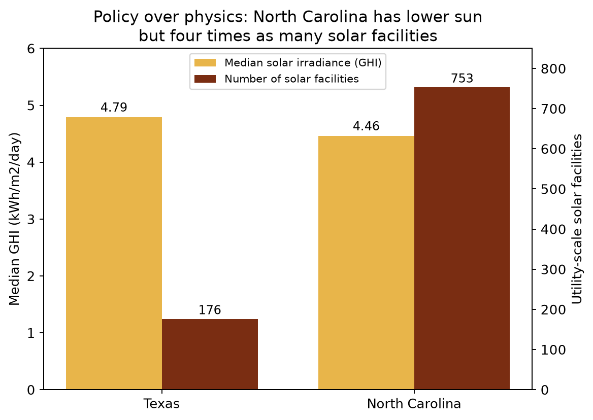
The siting rule holds in kind across both states but shifts in degree, and the shift tracks each state's policy regime rather than its irradiance. Comparable siting papers rarely test transfer at all.
Siting features are spatially autocorrelated, and naive random cross-validation leaks that structure and inflates scores. I report the full ladder instead of one number. Performance degrades gradually as the model generalizes further, and the large drop appears only at the state boundary.
| Validation | ROC-AUC | What it tests |
|---|---|---|
| Random CV | ~0.93 | Interpolation (optimistic) |
| Spatial block CV (130 km) | 0.92 | Spatial independence |
| Leave-one-region-out | 0.91 | Unseen Texas ecoregions |
| Transfer to North Carolina | 0.76 | Cross-state, cross-regime |
I set the block size from the measured 12 km residual autocorrelation range in the data. The leave-one-region-out test holds out entire EPA ecoregions in turn; at 0.91, the model generalizes across Texas geography instead of memorizing local quirks.
I checked the map's Area of Applicability (94.8% of Texas) against local data-point density: 86% of in-domain cells rest on 10 or more supporting training points.
- Circularity. The most obvious objection is that operating farms are wired to the grid by definition. I bounded this by removing every grid feature and retraining on interconnection-immune features only (irradiance, slope, elevation, land cover). The model still discriminates at ROC 0.72, so about two-thirds of the signal survives without any grid information. Grid access amplifies a pre-existing siting signal; it does not create one.
- Irradiance resolution. Coarse GHI could in principle make irradiance look unimportant. If anything the bias runs the other way: impurity importance favors high-cardinality features, penalizing coarse GHI. Under permutation importance it still ranks far below grid access, and Boruta keeps it as a real but minor predictor.
- Run-to-run stability. Across 10 replicate draws, transmission is the top feature in all 10 and substation second in all 10.
- Transfer stability. The North Carolina score holds at 0.76 ± 0.01 across 10 pseudo-absence draws.
I framed the problem as presence-background, borrowed from species distribution modeling: verified facilities versus pseudo-absences drawn from developable land, with 10 balanced replicate draws averaged for stability. Each facility is summarized over its actual footprint rather than a centroid, so a 500 MW plant is represented by the land it occupies. Features span irradiance (NREL/NSRDB), slope and elevation (USGS 3DEP), land cover (NLCD), and distance to transmission, substations, and roads (HIFLD, TIGER). A developable-land mask excludes steep, wet, forested, and densely built terrain following NREL and peer-reviewed conventions; it leaves 73.9% of Texas as candidate area.
The pipeline needed debugging along the way. The first assembled model table had a join bug that produced null features, and an early land-cover feature averaged categorical class codes into meaningless fractional values; I re-derived it as the integer mode. Before modeling I ran a full integrity audit script (src/99_audit.py) on the final table: 1,936 rows, 0 nulls. Method choices and their sources are documented in each script's header.
- Single training state and a modest sample (176 facilities). Texas is one regime; the North Carolina transfer probes generalization but does not replace multi-state training.
- The "irradiance is minor" claim is Texas-specific. Within a narrow, uniformly high irradiance range there is little gradient to track, so this says nothing about irradiance elsewhere.
- Suitability outputs are relative percentiles. Presence-background models recover relative suitability and discrimination rather than calibrated build probabilities.
- The panhandle (High Plains) is where the model extrapolates least well.
Open the code
Python pipeline, figures, and documentation on GitHub.