This pipeline has two distinct stages, both documented here in full:
- Stage A — point-cloud processing (ArcGIS Pro): raw LiDAR → 1 m DSM and DTM with verified coordinate handling (sections 02–04).
- Stage B — analytical pipeline (Python): the DSM → slope and aspect → per-building zonal aggregation → energy estimate, written with rasterio, geopandas, and NumPy (sections 05–07).
The same Python module runs both study areas — only the input surface changes — which is what makes the Austin/Kathmandu comparison a true methods transfer.
Source data: USGS 3DEP Lidar Point Cloud, project TX Central B1 2017, tile over the West Austin Neighborhood Group — 24,579,588 points, retrieved as a compressed LAZ file via the USGS 3DEP LidarExplorer.
ArcGIS Pro's Create LAS Dataset rejected the compressed .laz directly (Error 000814), so Convert LAS was used to decompress to .las and build the LAS dataset in one step. Two rasters were then produced with LAS Dataset To Raster, differing only in which returns are used and how cells are populated.
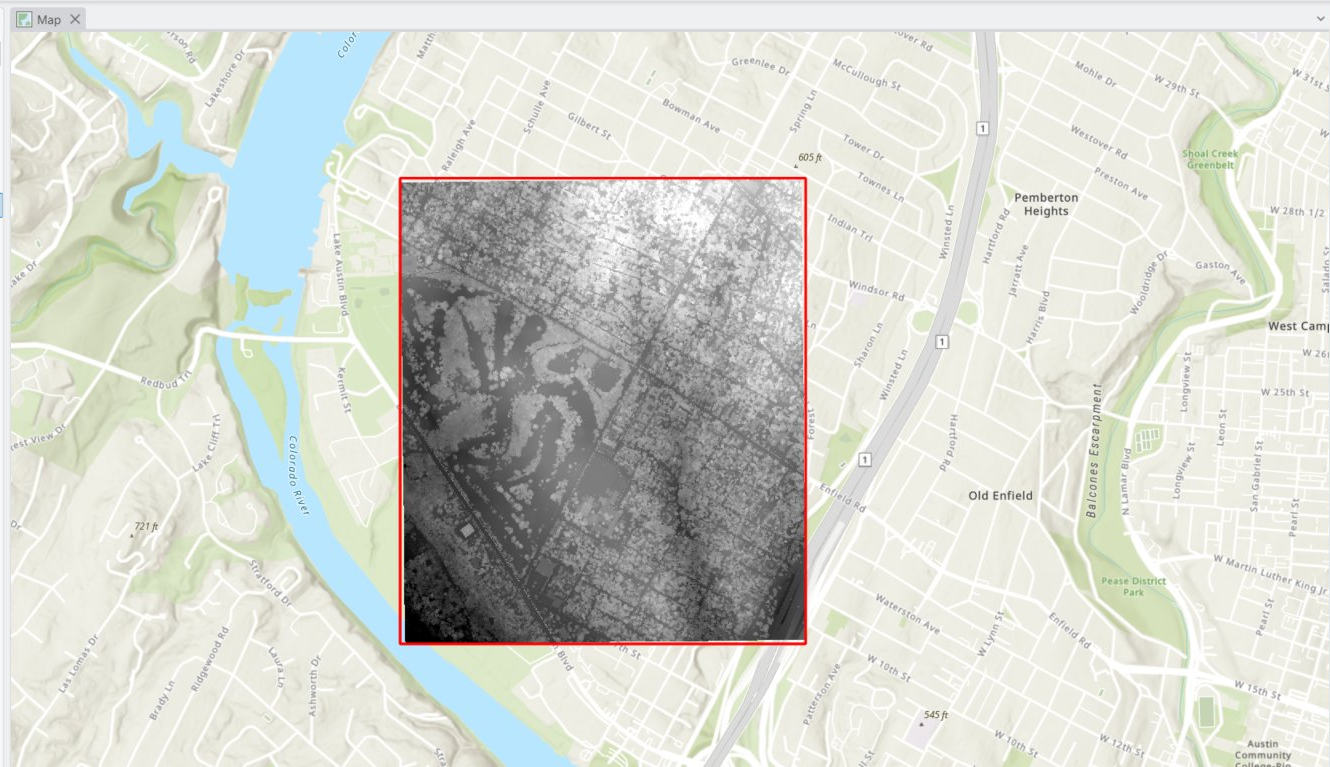
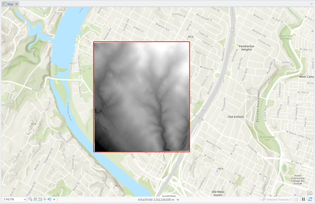
The DSM uses all returns, Maximum cell assignment (captures rooftop tops); the DTM uses ground-class returns, Minimum assignment (bare earth). The DSM range (130.7–254.3 m) versus the DTM range (130.9–187.9 m) confirms above-ground features were removed.
Correct CRS handling is essential — a misread of horizontal or vertical units would corrupt every slope and area calculation downstream.
- Projected CRS: NAD83(2011) / UTM Zone 14N (EPSG 6343), linear unit metres.
- Vertical CRS: NAVD88 height, unit metres.
- Implication: both horizontal and vertical are metres, so slope (degrees) and area (m²) compute directly with no unit conversion. EPSG 6343 was carried through to the Python analysis.
| Parameter | DSM (surface) | DTM (bare earth) |
|---|---|---|
| Tool | LAS Dataset To Raster | LAS Dataset To Raster |
| LAS filter | All returns | Ground class only |
| Interpolation | Binning | Binning |
| Cell assignment | Maximum | Minimum |
| Void fill | Linear | Linear |
| Cell size | 1 m | 1 m |
With the 1 m DSM in hand, the Python stage begins. Slope and aspect are derived directly from the elevation grid using the Horn (1981) 3×3 gradient — the same algorithm ArcGIS uses internally — rather than relying on a black-box tool. The raster is read with rasterio, nodata is masked to NaN, and the gradient is divided by the true pixel size so slope is in real degrees regardless of cell resolution.
# Horn 3x3 gradient — slope & aspect in degrees from any DSM
z = src.read(1).astype("float64"); z[z == src.nodata] = np.nan
dzdx = np.gradient(z, axis=1) / px      # divide by true pixel size (m)
dzdy = np.gradient(z, axis=0) / py
slope  = np.degrees(np.arctan(np.sqrt(dzdx**2 + dzdy**2)))
aspect = np.degrees(np.arctan2(dzdy, -dzdx))   # compass-corrected below
src/solar_suitability.py · slope_aspect() — vectorised over the whole grid with NumPy (no Python loops).
OpenStreetMap building footprints are pulled with osmnx and reprojected to the DSM's CRS with geopandas. For each footprint, rasterio's geometry_mask rasterises the polygon into a boolean mask over the slope/aspect grids — a true zonal-statistics operation done in-memory. Cells under the slope cap define the usable fraction; the equator-facing aspect score is averaged only over those usable cells.
# For each OSM footprint: mask the raster & reduce to usable stats
mask = geometry_mask([geom], out_shape=slope.shape,
                     transform=transform, invert=True)
s, a = slope[mask], aspect[mask]                 # cells inside this roof
under_cap   = s <= max_slope_deg                  # slope usability filter
frac_usable = under_cap.mean()                  # fraction of roof mountable
aspect_score = _aspect_score(a[under_cap]).mean()  # 1.0 = faces equator
src/solar_suitability.py · building_suitability() — geometry-aware reduction, not a generic raster average.
The annual per-building yield is a transparent, first-order model — every term is explicit and defensible, with no hidden coefficients:
# Transparent energy model — every factor is explicit
usable_area = footprint_area * usable_fraction * frac_usable   # m²
annual_kwh  = (usable_area * annual_ghi_kwh_m2 * aspect_score
               * panel_efficiency * performance_ratio)         # kWh/yr
usable_fraction (mountable share), GHI (irradiation), panel efficiency, performance ratio — all named parameters.
The Kathmandu transfer adds one Python step the LiDAR side did not need: the open Copernicus DSM arrives in geographic WGS84 (degrees), so it is reprojected to metric UTM 45N with rasterio's calculate_default_transform and reproject before the identical analysis runs — guaranteeing slope and area are computed in metres for both cities.
The point-cloud stage ran in the ArcGIS Pro GUI — a standard professional workflow documented here by tool and parameter. From the DSM onward, every step is scripted, vectorised, and reproducible from the repository: one shared module, two cities.
See the analysis & code
The comparative analysis and the full reproducible pipeline.