| Metric | Austin · 1 m LiDAR | Kathmandu · 30 m DSM |
|---|---|---|
| Elevation source | USGS 3DEP LiDAR | Copernicus GLO-30 |
| OSM footprints fetched | 1,795 | 7,290 |
| Buildings analyzed | 1,728 | 947 |
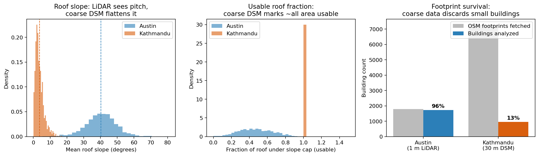
| Footprint survival | 96.3% | 13.0% |
| Mean roof slope | 40.3° | 3.7° |
| Usable roof fraction | 0.47 | 1.00 |
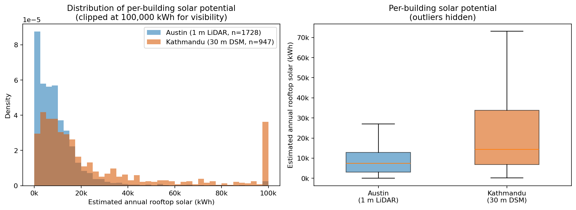
| Median kWh / building | 7,404 | 14,355 |
| Total annual kWh | 19,187,570 | 36,256,333 |
The two cities' per-building distributions are statistically distinct. A Mann–Whitney U test rejects equal distributions (p ≈ 10⁻⁶⁸) and a Kolmogorov–Smirnov test confirms a large separation (D = 0.31).
Counter-intuitively, Kathmandu's median per-building estimate (14,355 kWh) is nearly double Austin's (7,404 kWh) — despite Kathmandu's buildings being physically smaller. Section 03 explains why this is an artifact, not a real difference.
Coarse open data adds directional bias, via two compounding mechanisms:
- Roof-pitch flattening. At 1 m, LiDAR resolves individual roof planes (mean slope 40.3°, only 47% of area usable). At 30 m, one cell spans an entire small building, averaging pitched surfaces into a near-flat patch (slope 3.7°, 100% usable). The coarse DSM cannot see that roofs are tilted, so it over-credits usable area.
- Small-building dropout. A 30 m cell is larger than many Kathmandu buildings; footprints with too few valid cells are dropped. Only 13% of fetched footprints survive, biasing the sample toward large, high-yield structures.
Building footprint area correlates strongly with estimated yield (Pearson r = 0.98 Austin, 0.92 Kathmandu), confirming usable area is the dominant driver — exactly the quantity the coarse DSM distorts.
Airborne LiDAR (Austin)
- Resolves roof planes — true per-facet slope, aspect, usable area.
- High footprint survival; nearly all buildings analyzable.
- Not openly available for most of the world; large, heavier to process.
Open global DSM (Kathmandu)
- Globally available, free, fast — the only option where LiDAR is absent.
- Adequate for coarse screening of districts and large rooftops.
- Cannot resolve roof planes; flattens pitch, over-credits usable area, drops small buildings.
- Per-building values are a relative screen, not absolute design figures.
- Irradiation values are placeholders (Austin 1,700; Kathmandu 1,800 kWh/m²/yr); absolute totals are provisional, relative within-city rankings robust.
- Kathmandu is a footprint-level screen at 30 m, not roof-facet design.
- First-order energy model; no inter-building shading in the Python step.
- OSM footprint completeness and the choice of footprint dataset materially affect Kathmandu totals.
See how the LiDAR was processed
The full point-cloud-to-surface methodology, and the reproducible code.